Comparison of Computational Complexity and Accuracy for Focus Algorithm Implemented Within a Field Programmable Gate Array.
June, 2015Timothy Duffy Rochester Intitute of Technology tim@timduffy.me
Clark Hochgraf Rochester Intitute of Technology cghiee@rit.edu
Abstract
Field Programmable Gate Arrays (FPGA) have found a strong and permanent home in the world of image processing. Their highly configurable nature allows for integration of almost any imager interface, while allowing for implementation of highly paralleled processing of algorithms. A current drawback of commercial FPGA devices is the lack of hardened Floating Point math primitives. This limitation prevents the size-efficient implementation of some algorithms, specifically those dealing with frequency domain conversion. A comparison is done against four different focus calculation algorithms across three different Region of Interest (ROI) sizes, to determine if a purely spacial domain calculation could be accomplished to reduce the amount of logic required within the FPGA fabric. Reducing the amount of logic used, and increasing the speed at which the RTL runs, allows for a reduction in cost, and an increase in the range of image sizes the hardware can support. It was determined that a simple side-by-side pixel difference was the most efficient use of the FPGA fabric, while producing repeatable, accurate results.
Introduction
FPGA technology is highly suited for image processing applications due to its highly parallel nature. FPGA integrated circuits provide a large amount of configurable logic that can be used to implement a wide range of different image processing algorithms from edge detection, sharpening, object detection, pattern matching, color space conversion, etc. Many of these images require a highly focused image to work correctly. Great care is taken to provide the highest quality image from imaging systems today, as well as large amounts of research that is done to produce the algorithms that consume those images.
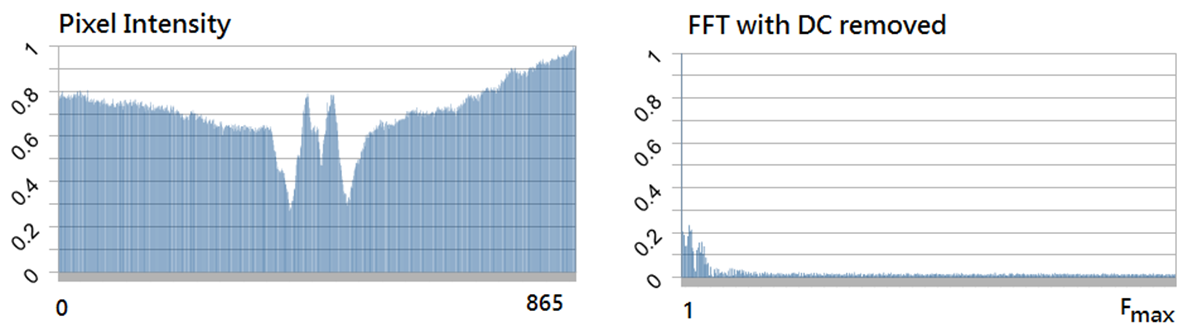
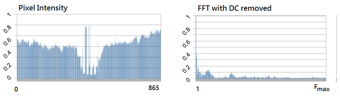
Focus of an image can be defined as the image within a set that has the largest sum of differences between the intensity of its pixels in the spacial domain, or the largest amount of energy within the image in the frequency domain.
Most imaging systems produce information that exists within the spacial domain, and if the target algorithms won't deal with data within the frequency domain, a conversion is undesirable from a computational complexity and cost. Due to the identified computational complexities of frequency domain conversion, finding the most focused image out of the image set using the time domain is preferable.
This paper will investigate four different methods of determining the most focused image within an image set across three different sized ROI and four different data sets.
Theory of Operation
The intensity of an imaging system can be determined in a number of different ways. In the case of a monochrome image, each pixel value is the image's intensity. In the case of a NTSC video stream, intensity is represented by the Y value. In a RGB color space, the intensity is determined by the ratio of red, green, and blue sensitive pixels, and their level of sensitivity within their color band.
The difference between two side-by-side pixels can be used as a method to determine the amount of sharpness, or energy an image has. The larger the difference, that is the sharper the image, the more energy the image has, and thus the more focused the image can be said to be. Out of focus images will have more pixels whose values are closer to their neighbor than those within a more focused image. Blurring within an image (out of focus) comes from the lens system's focal point not being on the imaging device's focal plane.
System Requirements
A low-cost hardware platform for assisting individuals with the degenerative eye disease Macular Degeneration was designed using a primitive, plastic lens system, a sub-megapixel camera, a small FPGA, and two near-eye displays. The device works by being placed over an individual's eyes, and worn like a large pair of classes. The device provides near-vision assistance by applying a number of algorithms to the video stream becore displaying it to the user. Due to the price sensitivity of the platform, very efficient use of the FPGA fabric was required as not to require a larger FPGA device, which would increase the cost of other parts of the support system such as power supplies.
Most of the algorithms within the system require a maximally focused image to perform optimally, or at all. It was determined via testing that an automatic focus system would be required to ensure the most focused image was presented to the image processing device.
It was identified that the existing, competitive, products took far too long to find focus. This proved to be a point of frustration for the intended audience of older, non-technology savy individuals. It was determined that focus should be found within one second to reduce confusion and frustration with the device.
Due to the time requirement of one second, it was determined that calculating a focus value for each frame would be necessary. A definition of the maximally focused frame was defined as the image that produced the largest summation of differences between pixels, or the largest amount of energy within the frame.
Data Sets
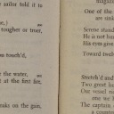
Four focus calculation methods were investigated. Four different image sets were used against all four methods. Those data sets can be seen in Figures 1, 2, 3, and 4. Each image within the four data sets were 865x577 pixels, a total of 499,105 pixels per image. When the image data sets were captured, the center image of the set was set as the approximate maximally focused image. This was done for demonstration purposes only and does not reflect in-field datasets.
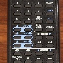
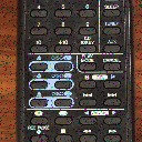
All four methods take a centered ROI within the image as their input. An example of one of these ROI segments can be seen in Figure 2 and Figure 3 . Each of the four image sets were used to create a companion data set with salt and pepper noise added to assist with proving out algorithm robustness. The implementation of this can be seen in Appendix A.


Due to electrical noise introduced by the low-cost lens system, an image could not be captured while the lens system was moving. Lens movement was thus performed during the blanking sections of each frame read-out of the imager. This movement occurred within less than 10 milliseconds, and happened at a maximum of 30 times per second, as the imager ran at 30 frames per second, with approximately 30 percent blanking time. While the lens system was moving during the imager blanking time the focus calculation was performed and the system prepared for the next frame to arrive.
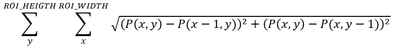
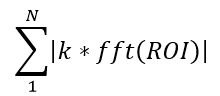
Methods
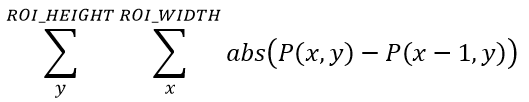
A summation side-by-side pixel difference method (seen in Equation 1), a summation of vertical and horizontal pixel difference method (seen in Equation 2), a single dimension FFT method (seen in Equation 3), and a two dimensional FFT method (seen in Equation 4) were implemented within GUI Octave and then VHDL.

Findings
After implementing the four focus algorithms within GNU Octave, it was found that an ROI of 32x32 pixels was not enough information to produce a usable image set. 128X128 pixels was determined to be a sufficient amount of information for the focus algorithms to work reliably and repeatable. Table 1 shows the RIO sizes used.
| ROI Size | Number of Pixels | Percentage of Image |
|---|---|---|
| 32x32 | 1024 | 0.20% |
| 64x64 | 4096 | 0.80% |
| 128x128 | 16384 | 3.00% |
The focus values produced by each equation was plotted on a graph, with the maximum value relative to the data set for each of the algorithms representing the most focused image. The results of these images can be seen in Figures 6, 7, 8, and 9 for the image sets for the book, business card, playing card, and television remote .
Motion blur was identified as a concern when gathering image data sets. Low-light conditions, resulting in higher integration times per pixel, generates motion blur within the image if the device is not kept completely still. This low-light sensitivity is a result of the inexpensive, plastic lens system chosen for the imaging system. Accessibly, in the form of low cost, to the product was given a higher weight than low-light operation, and thus a well-lit environment is necessary for the device to successfully find focus, as well as general operation to be performed correctly.
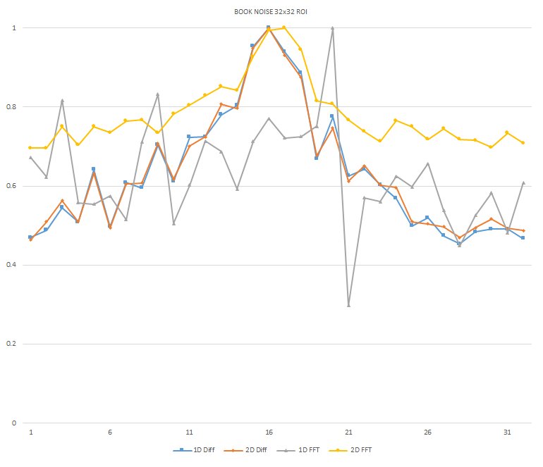
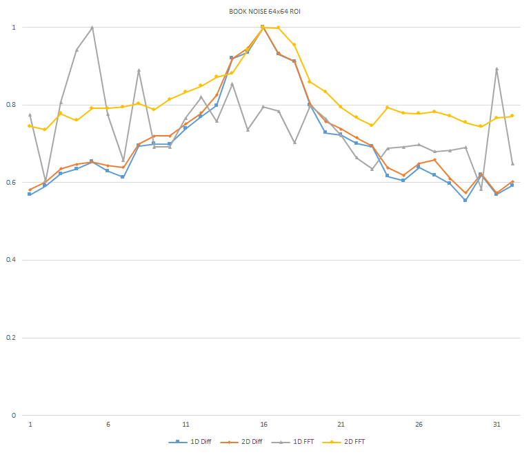
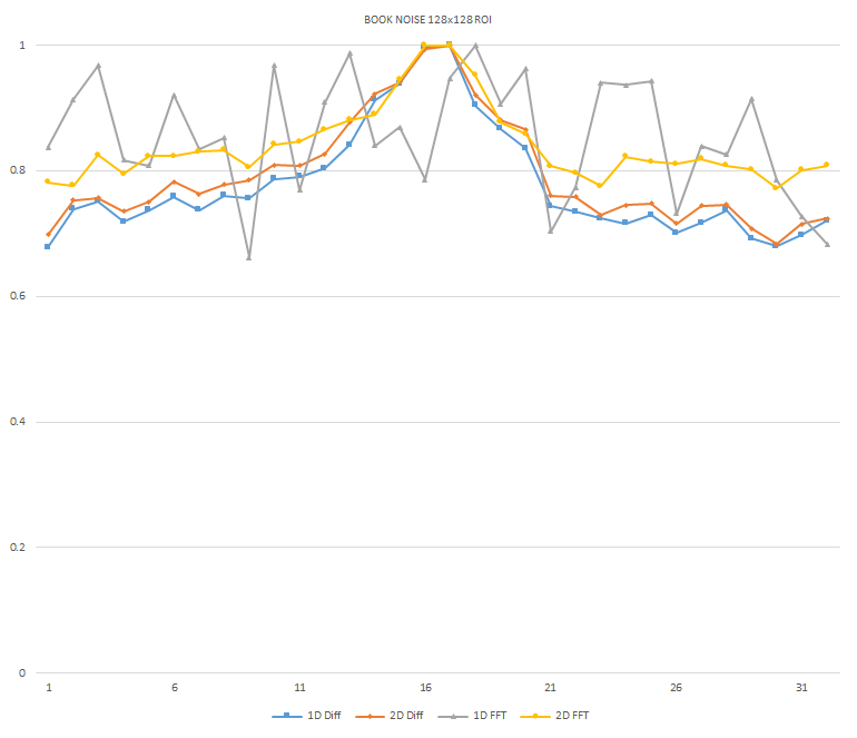
Book Image Set
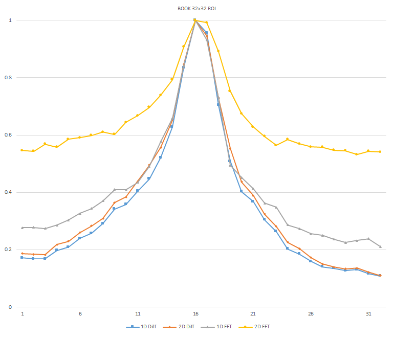
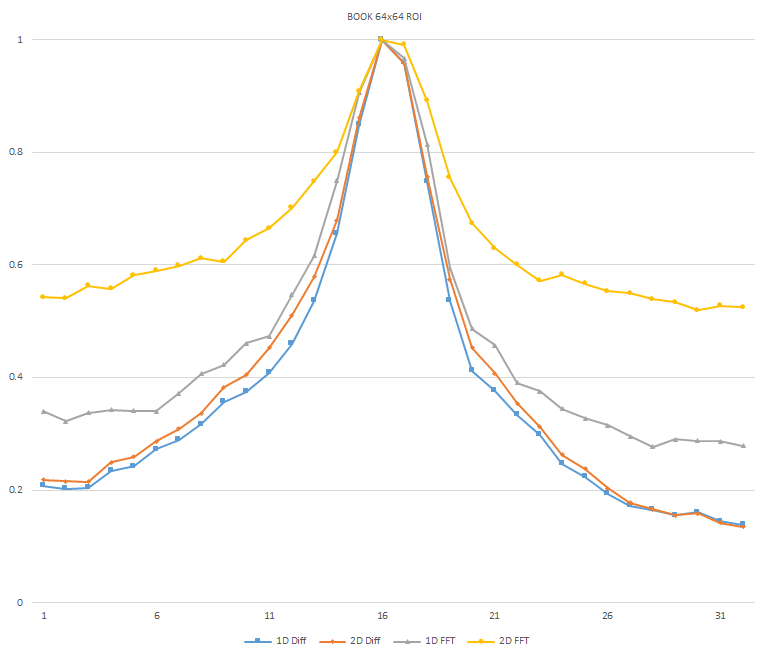
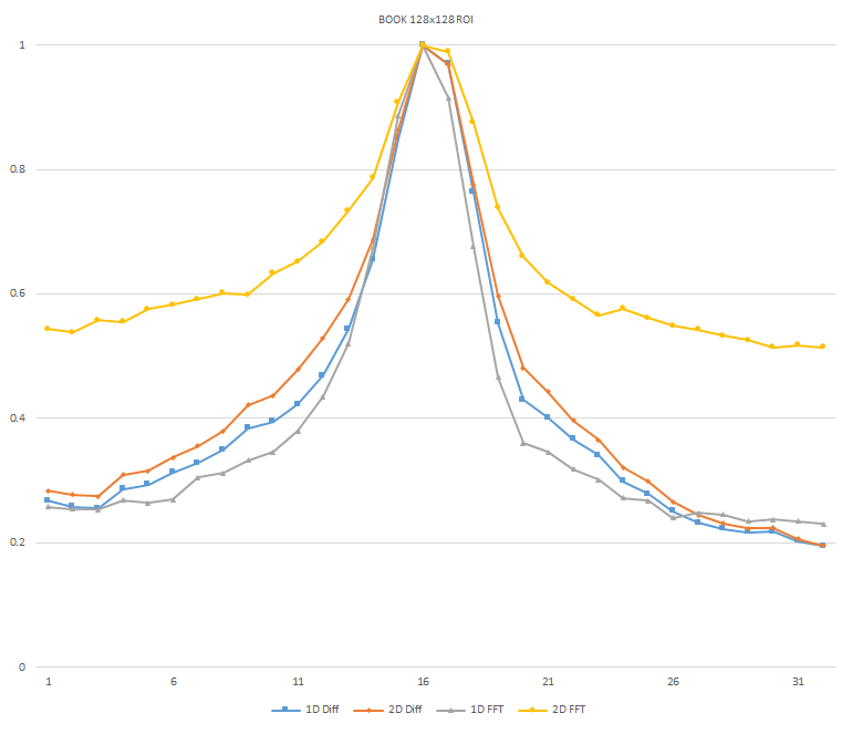
 Normalized focused level across the three different ROI sizes and four different target algorithms
for the Book image set. (a) 32x32 ROI, (b) 64x64 ROI, (c) 128x128 ROI, (d) noisy images 32x32 ROI, (e) noisy
images 64x64 ROI, (f) noisy images 128x128.
Normalized focused level across the three different ROI sizes and four different target algorithms
for the Book image set. (a) 32x32 ROI, (b) 64x64 ROI, (c) 128x128 ROI, (d) noisy images 32x32 ROI, (e) noisy
images 64x64 ROI, (f) noisy images 128x128.
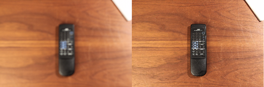
Remote Image Set
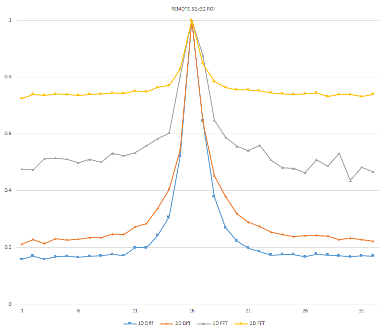
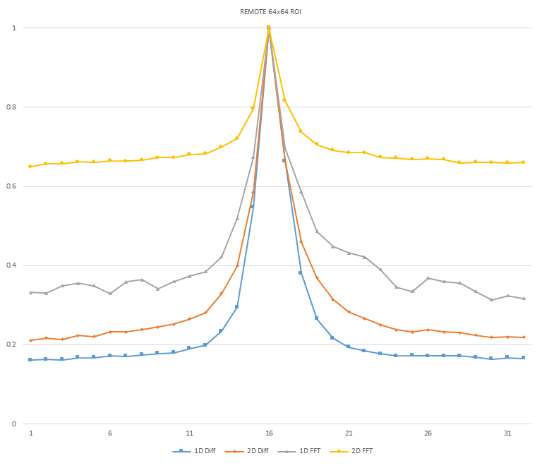
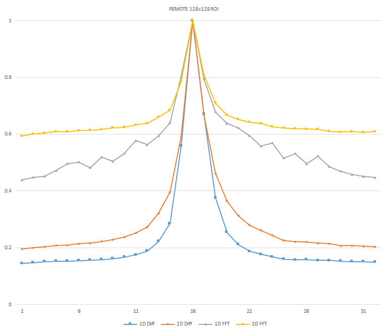
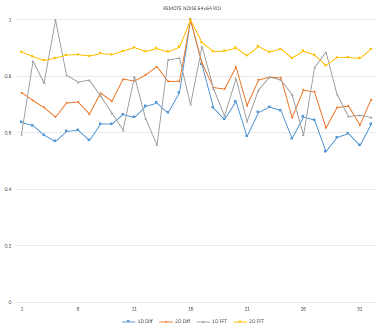
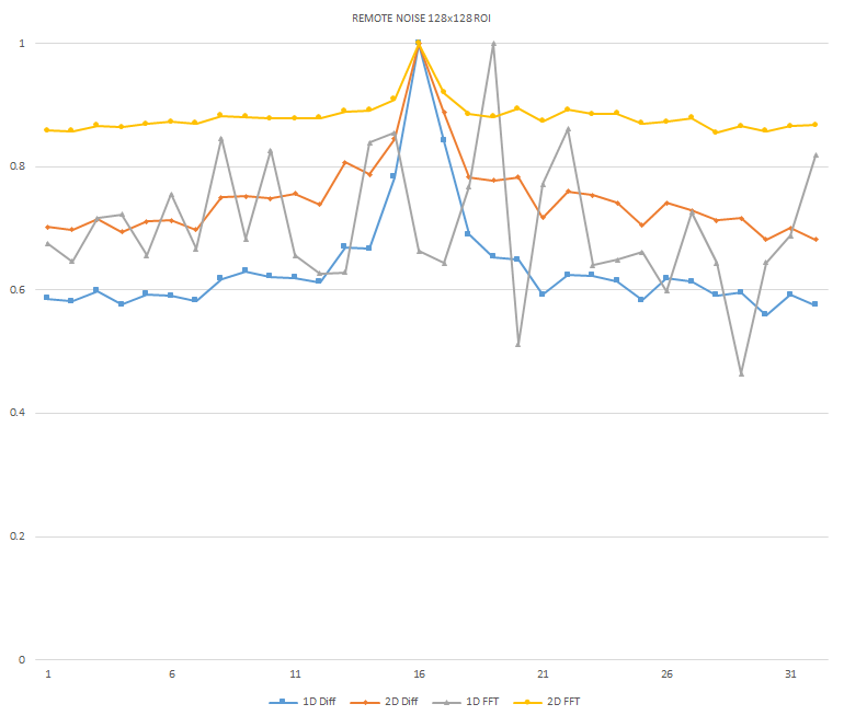 Normalized focused level across the three different ROI sizes and four different target algorithms for
the Remote image set. (a) 32x32 ROI, (b) 64x64 ROI, (c) 128x128 ROI, (d) noisy images 32x32 ROI, (e)
noisy images 64x64 ROI, (f) noisy images 128x128.
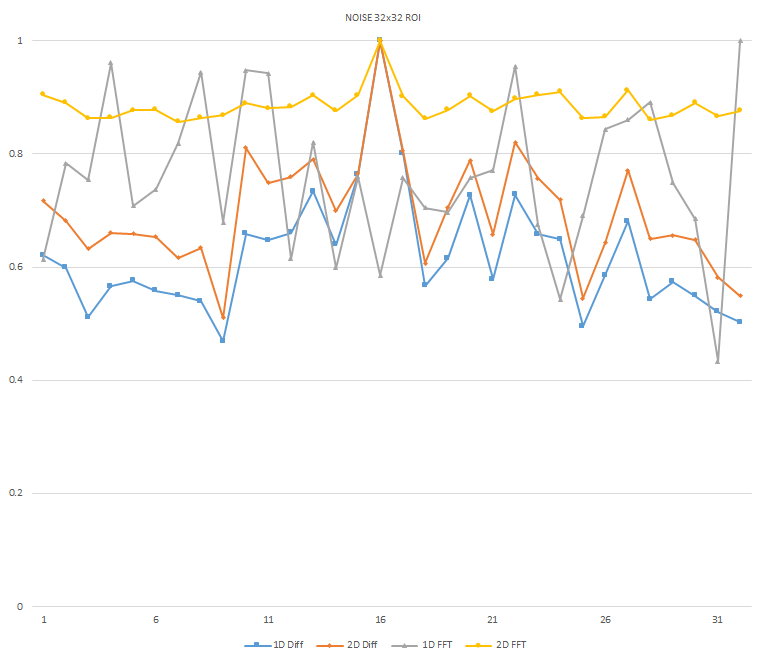
Normalized focused level across the three different ROI sizes and four different target algorithms for
the Remote image set. (a) 32x32 ROI, (b) 64x64 ROI, (c) 128x128 ROI, (d) noisy images 32x32 ROI, (e)
noisy images 64x64 ROI, (f) noisy images 128x128.
Business Card Image Set
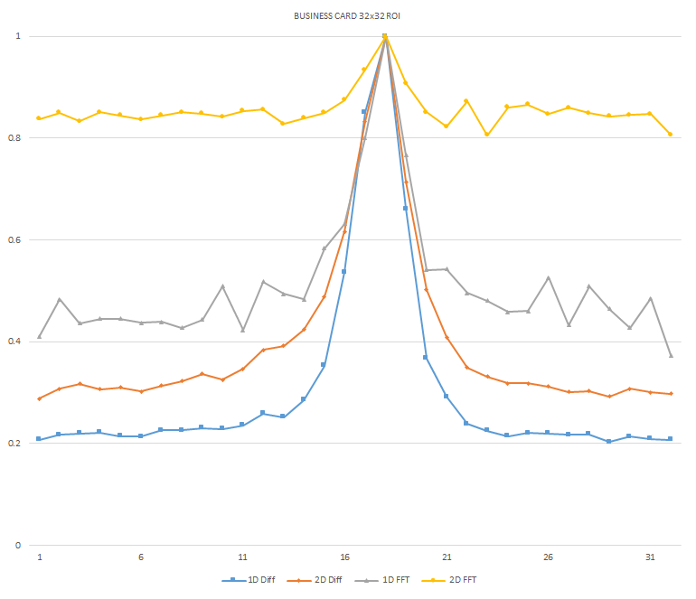
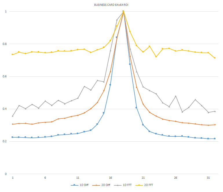
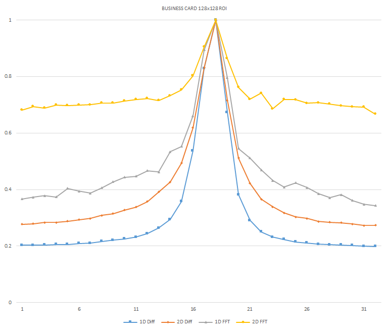
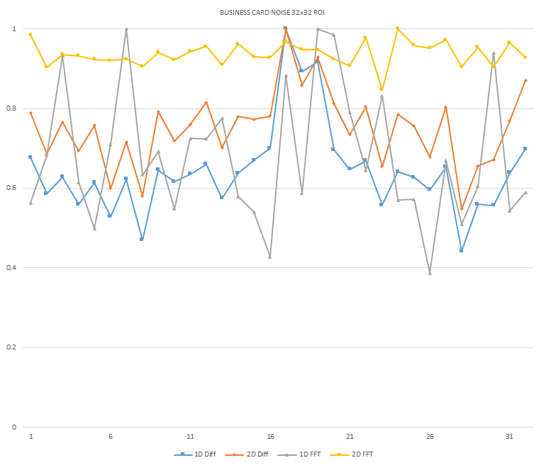
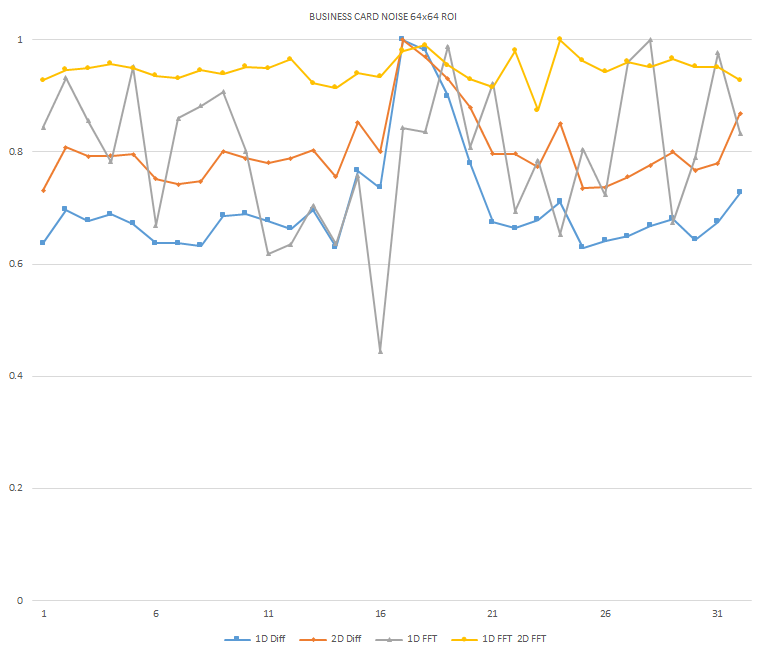
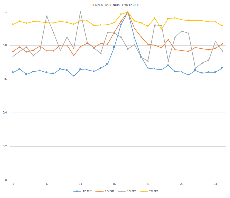 Normalized focused level across the three different ROI sizes and four different target algorithms
for the Business Card image set. (a) 32x32 ROI, (b) 64x64 ROI, (c) 128x128 ROI, (d) noisy images 32x32
ROI, (e) noisy images 64x64 ROI, (f) noisy images 128x128.
Normalized focused level across the three different ROI sizes and four different target algorithms
for the Business Card image set. (a) 32x32 ROI, (b) 64x64 ROI, (c) 128x128 ROI, (d) noisy images 32x32
ROI, (e) noisy images 64x64 ROI, (f) noisy images 128x128.
Playing Card Image Set
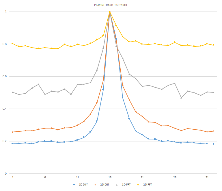
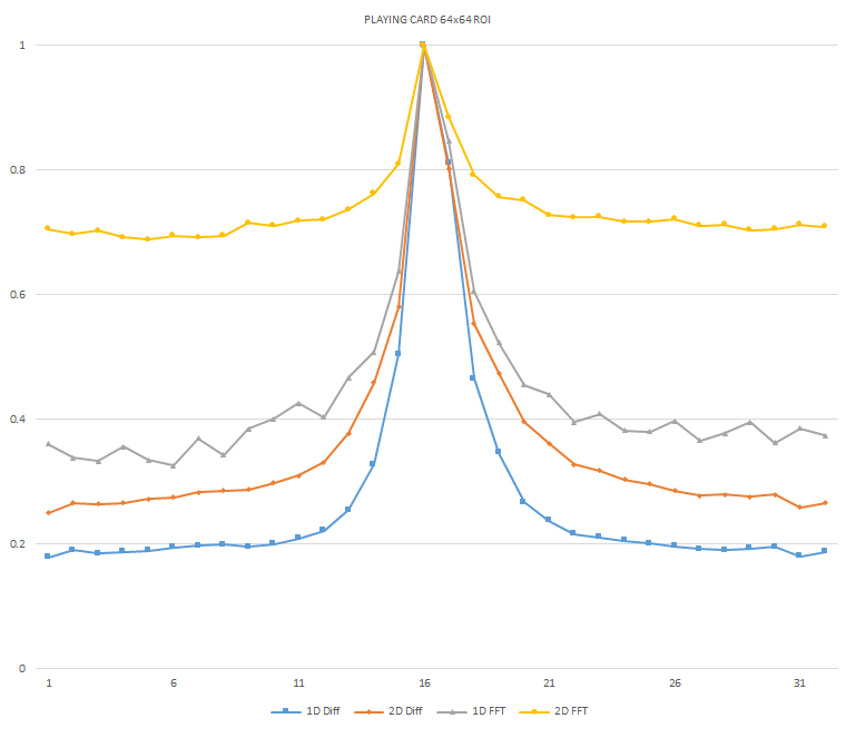
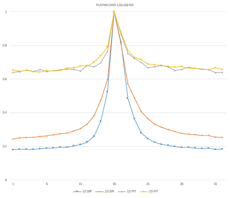
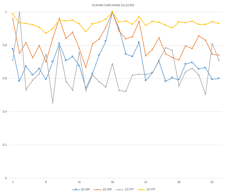
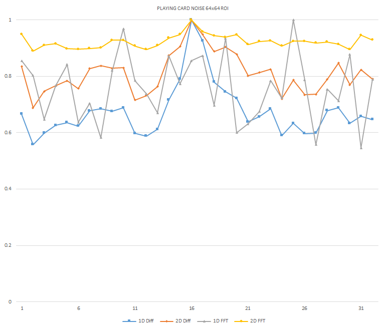
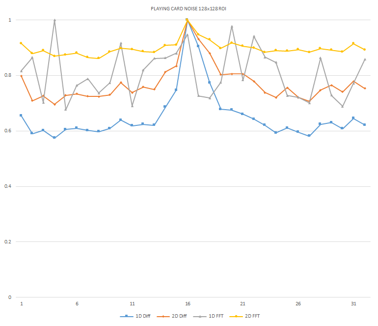 Normalized focused level across the three different ROI sizes and four different target algorithms
for the Playing Card image set. (a) 32x32 ROI, (b) 64x64 ROI, (c) 128x128 ROI, (d) noisy images 32x32
ROI, (e) noisy images 64x64 ROI, (f) noisy images 128x128.
Normalized focused level across the three different ROI sizes and four different target algorithms
for the Playing Card image set. (a) 32x32 ROI, (b) 64x64 ROI, (c) 128x128 ROI, (d) noisy images 32x32
ROI, (e) noisy images 64x64 ROI, (f) noisy images 128x128.
Business Card Image Set
Normalized focused level across the three different ROI sizes and four different target algorithms
for the Business Card image set. (a) 32x32 ROI, (b) 64x64 ROI, (c) 128x128 ROI, (d) noisy images 32x32
ROI, (e) noisy images 64x64 ROI, (f) noisy images 128x128.
Playing Card Image Set
Normalized focused level across the three different ROI sizes and four different target algorithms
for the Playing Card image set. (a) 32x32 ROI, (b) 64x64 ROI, (c) 128x128 ROI, (d) noisy images 32x32
ROI, (e) noisy images 64x64 ROI, (f) noisy images 128x128.
It can be seen in the above figures that the larger 128x128 ROI produces a set with a larger range in the original dataset. For the book image set, both the original image and noisy image produced focus values that had a range of more than 25 percent. For the remainder of the datasets, although a highly reduced range, both pixel differencing algorithms can be seen to produce the correct answer even under the noise.
The noise floor within all of the noisy image sets is much larger than the original data sets. This reduced range can be seen across all of the graphs labeled d, e, and f. The 2D FFT and pixel difference methods were able to find the correct maximally focused image with a large enough ROI. This was due to the fact that the percentage of the introduced noise is reduced as the ROI gets larger, and thus the noise has less of an effect both on the summation of difference values in the case of the pixel difference methods, and on the frequencies summation in the energy calculation methods.
Results
The most focused image within the four data sets was determined by the operator. Through a review of the data produced by all four algorithms across the three RIO sizes, four data sets, (including respective generated companion image sets), it can be seen that the summation side-by-side pixel difference method is the most reliable, consistent, accurate, and produces the largest range. Additionally, it is the computationally least complex, thus requiring much less FPGA fabric which helps minimize cost of the hardware platform.
The 1D Difference algorithm was determined to be the best solution for the types of data sets being presented to the imaging system. The summation of vertical and horizontal pixel difference method was just as good as the side-by-side method, however requires additional computational complexity. It was found that the one dimensional FFT method was incredibly unreliable at this RIO size and image content for noisy images. The two dimensional FFT method was seen as just as successful as the summation side-by-side pixel difference method, however requires the conversion of the data set into the frequency domain, thus is significantly more computationally intensive. Note that if the data needed to be converted for other algorithms in the system, this would be a sufficient method.
The 2D FFT method was determined to be a reliable method of determining focus in addition to the side-by-side 1D pixel difference algorithm for both the original data set and the generated noisy image set. As seen in Figures x and y, there is sufficient additional frequency information present between the least and most focused images within the remote dataset. Due to the significant increase in complexity to perform the spacial to frequency domain conversion within the FPGA and the results of the 1D pixel difference method and the 2D FFT method both being reliable algorithms, the 1D pixel-difference was chosen as the best algorithm for implementation.
Implementation
All four algorithms were implemented in VHDL. System utilization and clock speed for the implementation can be see within Table 2. The VHDL code for the preferred 1D Difference pixel difference can be seen in Appendix E.
| Spartan-6 | Artix-7 | Spartan-6 | Artix-7 | |
| Slice Registers | 106 | 106 | 106 | 106 |
| Slice LUT | 132 | 120 | 104 | 104 |
| DSP48 Blocks | 0 | 0 | 1 | 1 |
| Memory Blocks | 0 | 0 | 0 | 0 |
| Frequency | 190MHz | 267MHz | 93MHz | 143MHz |
(2) Maximum operating frequency is approximate based on Xilinx Datasheet DS260
The 1D and 2D FFT methods were not implemented within the FPGA, as their minimum requirements for FPGA resources were larger than the target FPGA device. The 2D FFT was seen as being a viable solution for all images within the datasets with ROI's of 64x64 pixels and bigger. Although robust with a smaller ROI, its implementation size prevented it from being a viable solution for this application. Additionally, the latency introduced by the FFT would cause a focus value to be generated every frame, however a frame delayed. This latency would prevent the lens system from moving each frame, as with the pixel-difference methods.
The selective nature of the 1D FFT implementation, where large portions of the ROI are not seen by the algorithm, was determined to be very unreliable. The algorithm was identified as a possible candidate since it was smaller than the 2D implementation, but still used frequency content of the image rather than special content. After testing it was determined not to be a valid method of determining focus of an image.
Conclusions
Finding focus within an image set can be easily determined on an FPGA due to the sequential nature of streaming image data and the highly parallel naturenation of FPGA fabric. It was determined that using a very simple summation of pixel value difference can be used to produce the index of the most focused image within a set.
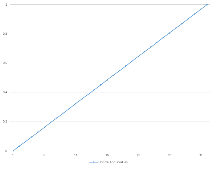
As seen in Figure xyz , an optimal output from the algorithm would be an increasing ramp, where each value is larger than the subsequent number. This would allow for the algorithm to quickly know if it is moving the lens system in the correct direction and getting closer to focus. As seen in the graphs of the different ROIs , there is little consistency between image sets. This level of inconsistency prevents the algorithm from intelligently determining which direction to move the lens without knowing the focus values at each focal step. Additionally, the noisy images show a large number of local-maxima which also proves difficult to make a direction estimation.
Since the imaging system has a sensitivity to low light environments, and the large amount of image variablily due to head motion by the operator, it was determined a full exhaustive search for the maximally focused image was necessary. Future work could be done to identify methods for direction prediction based on the existing hardware system. With a blurred image, a deconvolution can be performed to determine exactly where the lens needs to move.
Appendix A
All code for this project can be found here: Github.
Noisy Image Generation GNU Octave Code:
            function createNoisyImages(name)

                infolder = strcat("/cygdrive/c/dev/af_paper/images/",name,"/original/");
                outfolder = strcat("/cygdrive/c/dev/af_paper/images/",name,"/noise/");
                files = dir(infolder);

                for j = 3:length(files)
                    infilename = strcat(infolder,files(j).name);
                    img = imread(infilename);

                    % add noise to image
                    %outimg = imnoise(inimg,"salt & pepper",0.05);

                    a = 0.05;
                    noise = rand(size(img));
                    img(noise < a/2) = 0;
                    img(noise >= 1-a/2) = 1;

                    outfilename = strcat(outfolder,files(j).name);
                    imwrite(img,outfilename);
                end;

            endfunction;

            createNoisyImages('book');
            createNoisyImages('playing_card');
            createNoisyImages('remote');
            createNoisyImages('buisness_card');
Pixel summation VHDL code
                library IEEE;
                use IEEE.STD_LOGIC_1164.ALL;
                use IEEE.STD_LOGIC_UNSIGNED.ALL;
                use IEEE.NUMERIC_STD.ALL;

                entity focus_calculation_pixel_difference_2d is
                    Port ( i_clk : in  STD_LOGIC;
                           i_reset : in  STD_LOGIC;
                        i_framevalid : in  STD_LOGIC;
                        i_linevalid : in  STD_LOGIC;
                           i_Y : in  STD_LOGIC_VECTOR(7 downto 0);
                           --i_dv : in  STD_LOGIC;
                           o_focusvalue : out  STD_LOGIC_VECTOR (31 downto 0);
                           o_dv : out  STD_LOGIC);
                end focus_calculation_pixel_difference_2d;

                architecture Behavioral of focus_calculation_pixel_difference_2d is

                  --
                  -- images are 865x577
                  --
                  -- ROI box size is 128x128
                  --
                  -- (865/2) - (128/2) = 368, "0101110000" (note: -1 for inclusive)
                  -- (865/2) + (128/2) = 496, "0111110000" (note: +1 for inclusive)
                  -- (577/2) - (128/2) = 224, "0011100000" (note: -1 for inclusive)
                  -- (577/2) + (128/2) = 352, "0101100000" (note: +1 for inclusive)


                  constant C_STARTPIXELCOUNT : STD_LOGIC_VECTOR(9 downto 0) := "0101111110";
                  constant C_STOPPIXELCOUNT : STD_LOGIC_VECTOR(9 downto 0)  := "0111110001";
                  constant C_STARTLINECOUNT : STD_LOGIC_VECTOR(9 downto 0)  := "0011111110";
                  constant C_STOPLINECOUNT : STD_LOGIC_VECTOR(9 downto 0)   := "0101100001";

                  signal r_framevalidlast : STD_LOGIC;
                  signal r_linevalidlast : STD_LOGIC;
                  signal r_linecount : STD_LOGIC_VECTOR(9 downto 0);
                  signal r_pixelcount : STD_LOGIC_VECTOR(9 downto 0);
                  signal r_pixelvalid : STD_LOGIC := '0';
                  signal r_pixelvalid_last : STD_LOGIC := '0';

                  signal r_y : STD_LOGIC_VECTOR(7 downto 0);
                  signal r_y1 : STD_LOGIC_VECTOR(7 downto 0);

                  signal r_pixelsum : STD_LOGIC_VECTOR(31 downto 0);

                  signal r_dv :  STD_LOGIC;
                  signal r_focusvalue :  STD_LOGIC_VECTOR(31 downto 0);

                  type linetype is array( 0 to 128 ) of std_logic_vector(7 downto 0);
                  signal lastline : linetype := (others => "00000000");
                  --signal lineB : linetype;
                  --signal linepingpong : std_logic := '0';

                  signal roi_pixelcount : integer range 0 to 129 := 1;

                begin

                  o_focusvalue < r_focusvalue;
                  o_dv < r_dv;

                  process( i_clk )
                  begin
                    if ( rising_edge( i_clk ) ) then
                      if ( i_reset = '1' ) then

                        r_framevalidlast < '0';
                        r_linevalidlast < '0';
                      else

                        r_framevalidlast < i_framevalid;
                        r_linevalidlast < i_linevalid;
                      end if;
                    end if;
                  end process;

                  process( i_clk )
                  begin
                    if ( rising_edge( i_clk ) ) then
                      if ( i_reset = '1' ) then

                        r_Y < (others => '0');
                        r_Y1 < (others => '0');

                      else

                        -- delayed 2 clocks to compensate for r_pixelvalid calculation
                        r_Y < i_Y;
                        r_Y1 < r_Y;
                      end if;
                    end if;
                  end process;

                  -- linecount
                  process( i_clk )
                  begin
                    if ( rising_edge( i_clk ) ) then
                      if ( i_reset = '1' ) then
                        r_linecount < (others => '0');
                      else
                        r_linecount < r_linecount;
                        if ( r_framevalidlast = '0' and i_framevalid = '1' ) then
                          r_linecount < (others => '0');
                        elsif ( i_framevalid = '1' ) then
                          r_linecount < r_linecount + '1';
                        end if;
                      end if;
                    end if;
                  end process;

                  -- pixelcount
                  process( i_clk )
                  begin
                    if ( rising_edge( i_clk ) ) then
                      if ( i_reset = '1' ) then
                        r_pixelcount < (others => '0');
                      else
                        r_pixelcount < r_pixelcount;
                        if ( r_linevalidlast = '0' and i_linevalid = '1' ) then
                          r_pixelcount < (others => '0');
                        elsif ( i_framevalid = '1' ) then
                          r_pixelcount < r_pixelcount + '1';
                        end if;
                      end if;
                    end if;
                  end process;

                  process( i_clk )
                  begin
                    if ( rising_edge( i_clk ) ) then
                      if ( i_reset = '1' ) then
                      else
                        r_pixelvalid < '0';
                        if ( r_pixelcount > C_STARTPIXELCOUNT and r_pixelcount < C_STOPPIXELCOUNT and r_linecount > C_STARTLINECOUNT and r_linecount < C_STOPLINECOUNT ) then
                          r_pixelvalid < '1';
                        end if;
                        r_pixelvalid_last < r_pixelvalid;
                      end if;
                    end if;
                  end process;

                  -- pixelsum
                  process( i_clk )
                    variable xdiff : std_logic_vector(7 downto 0) := (others => '0');
                    variable ydiff : std_logic_vector(7 downto 0) := (others => '0');
                  begin
                    if ( rising_edge ( i_clk ) ) then
                      if ( i_reset = '1' ) then
                        r_pixelsum < (others => '0');
                        --roi_pixelcount < 1;
                      else

                        r_pixelsum < r_pixelsum;
                        --roi_pixelcount < roi_pixelcount;

                        if ( r_framevalidlast = '0' and i_framevalid = '1' ) and ( r_linevalidlast = '0' and i_linevalid = '1' ) then
                          r_pixelsum < (others => '0');
                        else
                          if ( r_pixelvalid = '1' ) then

                            if ( r_Y > r_Y1 ) then
                              xdiff := (r_Y - r_Y1);
                            else
                              xdiff := (r_Y1 - r_Y);
                            end if;

                            if ( lastline(roi_pixelcount-1) > r_Y1 ) then
                              ydiff := (lastline(roi_pixelcount-1) - r_Y1);
                            else
                              ydiff := (r_Y1 - lastline(roi_pixelcount-1));
                            end if;

                            r_pixelsum < r_pixelsum + ( ( xdiff * xdiff ) + ( xdiff * xdiff ) );

                            lastline(roi_pixelcount) < r_Y1;

                          end if;
                        end if;
                      end if;
                    end if;
                  end process;

                  process( i_clk )
                  begin
                    if ( rising_edge ( i_clk ) ) then
                      if ( i_reset = '1' ) then
                        roi_pixelcount < 1;
                      else

                        roi_pixelcount < roi_pixelcount;

                        if ( r_pixelvalid = '0' ) then
                          roi_pixelcount < 1;
                        end if;

                      end if;
                    end if;
                  end process;

                  process( i_clk )
                  begin
                    if ( rising_edge( i_clk ) ) then
                      if ( i_reset = '1' ) then
                        r_dv < '0';
                        r_focusvalue < (others => '0');
                      else
                        r_dv < '0';
                        r_focusvalue < r_focusvalue;
                        if ( r_pixelcount = C_STOPPIXELCOUNT and r_linecount = C_STOPLINECOUNT ) then
                          r_dv < '1';
                          r_focusvalue < r_pixelsum;
                        end if;
                      end if;
                    end if;
                  end process;
                end Behavioral;
function createNoisyImages(name)
infolder = strcat("/cygdrive/c/dev/af_paper/images/",name,"/original/");
outfolder = strcat("/cygdrive/c/dev/af_paper/images/",name,"/noise/");
files = dir(infolder);
for j = 3:length(files)
infilename = strcat(infolder,files(j).name);
img = imread(infilename);
% add noise to image
%outimg = imnoise(inimg,"salt & pepper",0.05);
a = 0.05;
noise = rand(size(img));
img(noise < a/2) = 0;
img(noise >= 1-a/2) = 1;
outfilename = strcat(outfolder,files(j).name);
imwrite(img,outfilename);
end;
endfunction;
createNoisyImages('book');
createNoisyImages('playing_card');
createNoisyImages('remote');
createNoisyImages('buisness_card');
library IEEE;
use IEEE.STD_LOGIC_1164.ALL;
use IEEE.STD_LOGIC_UNSIGNED.ALL;
use IEEE.NUMERIC_STD.ALL;
entity focus_calculation_pixel_difference_2d is
Port ( i_clk : in STD_LOGIC;
i_reset : in STD_LOGIC;
i_framevalid : in STD_LOGIC;
i_linevalid : in STD_LOGIC;
i_Y : in STD_LOGIC_VECTOR(7 downto 0);
--i_dv : in STD_LOGIC;
o_focusvalue : out STD_LOGIC_VECTOR (31 downto 0);
o_dv : out STD_LOGIC);
end focus_calculation_pixel_difference_2d;
architecture Behavioral of focus_calculation_pixel_difference_2d is
--
-- images are 865x577
--
-- ROI box size is 128x128
--
-- (865/2) - (128/2) = 368, "0101110000" (note: -1 for inclusive)
-- (865/2) + (128/2) = 496, "0111110000" (note: +1 for inclusive)
-- (577/2) - (128/2) = 224, "0011100000" (note: -1 for inclusive)
-- (577/2) + (128/2) = 352, "0101100000" (note: +1 for inclusive)
constant C_STARTPIXELCOUNT : STD_LOGIC_VECTOR(9 downto 0) := "0101111110";
constant C_STOPPIXELCOUNT : STD_LOGIC_VECTOR(9 downto 0) := "0111110001";
constant C_STARTLINECOUNT : STD_LOGIC_VECTOR(9 downto 0) := "0011111110";
constant C_STOPLINECOUNT : STD_LOGIC_VECTOR(9 downto 0) := "0101100001";
signal r_framevalidlast : STD_LOGIC;
signal r_linevalidlast : STD_LOGIC;
signal r_linecount : STD_LOGIC_VECTOR(9 downto 0);
signal r_pixelcount : STD_LOGIC_VECTOR(9 downto 0);
signal r_pixelvalid : STD_LOGIC := '0';
signal r_pixelvalid_last : STD_LOGIC := '0';
signal r_y : STD_LOGIC_VECTOR(7 downto 0);
signal r_y1 : STD_LOGIC_VECTOR(7 downto 0);
signal r_pixelsum : STD_LOGIC_VECTOR(31 downto 0);
signal r_dv : STD_LOGIC;
signal r_focusvalue : STD_LOGIC_VECTOR(31 downto 0);
type linetype is array( 0 to 128 ) of std_logic_vector(7 downto 0);
signal lastline : linetype := (others => "00000000");
--signal lineB : linetype;
--signal linepingpong : std_logic := '0';
signal roi_pixelcount : integer range 0 to 129 := 1;
begin
o_focusvalue < r_focusvalue;
o_dv < r_dv;
process( i_clk )
begin
if ( rising_edge( i_clk ) ) then
if ( i_reset = '1' ) then
r_framevalidlast < '0';
r_linevalidlast < '0';
else
r_framevalidlast < i_framevalid;
r_linevalidlast < i_linevalid;
end if;
end if;
end process;
process( i_clk )
begin
if ( rising_edge( i_clk ) ) then
if ( i_reset = '1' ) then
r_Y < (others => '0');
r_Y1 < (others => '0');
else
-- delayed 2 clocks to compensate for r_pixelvalid calculation
r_Y < i_Y;
r_Y1 < r_Y;
end if;
end if;
end process;
-- linecount
process( i_clk )
begin
if ( rising_edge( i_clk ) ) then
if ( i_reset = '1' ) then
r_linecount < (others => '0');
else
r_linecount < r_linecount;
if ( r_framevalidlast = '0' and i_framevalid = '1' ) then
r_linecount < (others => '0');
elsif ( i_framevalid = '1' ) then
r_linecount < r_linecount + '1';
end if;
end if;
end if;
end process;
-- pixelcount
process( i_clk )
begin
if ( rising_edge( i_clk ) ) then
if ( i_reset = '1' ) then
r_pixelcount < (others => '0');
else
r_pixelcount < r_pixelcount;
if ( r_linevalidlast = '0' and i_linevalid = '1' ) then
r_pixelcount < (others => '0');
elsif ( i_framevalid = '1' ) then
r_pixelcount < r_pixelcount + '1';
end if;
end if;
end if;
end process;
process( i_clk )
begin
if ( rising_edge( i_clk ) ) then
if ( i_reset = '1' ) then
else
r_pixelvalid < '0';
if ( r_pixelcount > C_STARTPIXELCOUNT and r_pixelcount < C_STOPPIXELCOUNT and r_linecount > C_STARTLINECOUNT and r_linecount < C_STOPLINECOUNT ) then
r_pixelvalid < '1';
end if;
r_pixelvalid_last < r_pixelvalid;
end if;
end if;
end process;
-- pixelsum
process( i_clk )
variable xdiff : std_logic_vector(7 downto 0) := (others => '0');
variable ydiff : std_logic_vector(7 downto 0) := (others => '0');
begin
if ( rising_edge ( i_clk ) ) then
if ( i_reset = '1' ) then
r_pixelsum < (others => '0');
--roi_pixelcount < 1;
else
r_pixelsum < r_pixelsum;
--roi_pixelcount < roi_pixelcount;
if ( r_framevalidlast = '0' and i_framevalid = '1' ) and ( r_linevalidlast = '0' and i_linevalid = '1' ) then
r_pixelsum < (others => '0');
else
if ( r_pixelvalid = '1' ) then
if ( r_Y > r_Y1 ) then
xdiff := (r_Y - r_Y1);
else
xdiff := (r_Y1 - r_Y);
end if;
if ( lastline(roi_pixelcount-1) > r_Y1 ) then
ydiff := (lastline(roi_pixelcount-1) - r_Y1);
else
ydiff := (r_Y1 - lastline(roi_pixelcount-1));
end if;
r_pixelsum < r_pixelsum + ( ( xdiff * xdiff ) + ( xdiff * xdiff ) );
lastline(roi_pixelcount) < r_Y1;
end if;
end if;
end if;
end if;
end process;
process( i_clk )
begin
if ( rising_edge ( i_clk ) ) then
if ( i_reset = '1' ) then
roi_pixelcount < 1;
else
roi_pixelcount < roi_pixelcount;
if ( r_pixelvalid = '0' ) then
roi_pixelcount < 1;
end if;
end if;
end if;
end process;
process( i_clk )
begin
if ( rising_edge( i_clk ) ) then
if ( i_reset = '1' ) then
r_dv < '0';
r_focusvalue < (others => '0');
else
r_dv < '0';
r_focusvalue < r_focusvalue;
if ( r_pixelcount = C_STOPPIXELCOUNT and r_linecount = C_STOPLINECOUNT ) then
r_dv < '1';
r_focusvalue < r_pixelsum;
end if;
end if;
end if;
end process;
end Behavioral;